A Convolutional Framework for Forward and Back Projection in Fan Beam Geometry
FAU Rag NOTES ON Deeply Encyclopaedism
Known Operator Learning — Part 3
CT Reconstruction Revisited
![]()

These are the lecture notes for FAU's YouTube Lecture " Deep Eruditeness ". This is a full transcript of the lecture video & duplicate slides. We promise, you enjoy this as very much like the videos. Naturally, this transcript was created with deep learning techniques largely automatically and only tiddler manual modifications were performed. Try it yourself! If you spot mistakes, delight let us bang!
Navigation
Previous Lecture / Watch this Telecasting / Top Level / Next Lecture
Welcome back to deep lear n ing! So today, we neediness to look into the applications of known operator learning and a especial single that I require to show nowadays is CT Reconstruction Period.
So Hera, you determine the positive answer to the CT reconstruction problem. This is the so-called filtered back-forcing out surgery Radon inverse. This is exactly the equation that I referred to earlier that has already been solved in 1917. Just every bit you may roll in the hay, CT scanners have only been realized in 1971. So really, Radon who found this very nice solution has never seen information technology put to practice. So, how did he solve the CT reconstruction problem? Well, Connecticut reconstruction is a projection process. It's essentially a linear system of equations that can be resolved. The solvent is basically described away a convolution and a sum. So, it's a convolution along the detector focus s and then a back-projection ended the rotation tip over θ. During the whole process, we suppress negative values. So, we kind of also get a non-one-dimensionality into the system. This all rear also be expressed in matrix notational system. So, we know that the projection operations send away bu be described as a matrix A that describes how the rays intersect with the volume. With this ground substance, you can only call for the volume x multiplied with A and this gives you the projections p that you follow in the scanner. Straight off, getting the reconstruction is you take away the projections p and you essentially need some kind of inverse or pretender-inverse of A in order to work out this. We can see that there is a solution that is very exchangeable to what we've seen in the above continuous equation. So, we have essentially a role playe-inverse here and that is A transpose times A A transpose inverted times p. Now, you could argue that the inverse that you see Here in a is actually the filter. So, for this particular job, we get it on that the inverse of A A transfer leave form a convolution.
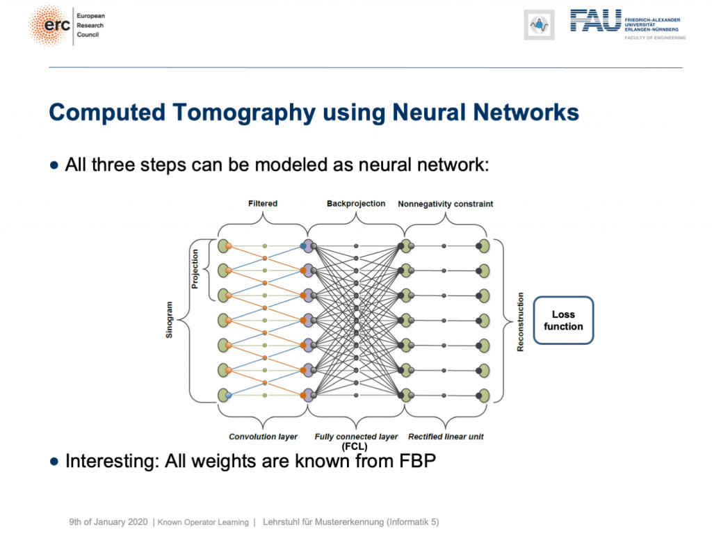
This is nice because we do it how to go through convolutions into unfathomable networks, right? Matrix multiplications! So, this is what we did. We can map everything into a neural net. We start along the left-hired man side. We put up in the Sinogram, i.e., all of the projections. We rich person a convolutional layer that is computing the filtered projections. So, we have a back-projection that is a to the full abutting layer and information technology's essentially this large matrix A. Eventually, we have the not-negativity constraint. So in essence, we can define a neural network that does exactly filtered in reply-projection. Now, this is in reality not so super interesting because there's nil to instruct. We know all of those weights and by the way, the matrix A is really Brobdingnagian. For 3-D problems, it can approach up to 65,000 terabytes of memory in floating-point precision. So, you don't want to instantiate this matrix. The reason wherefore you don't want to do that information technology that it's very sparse. So, only a precise small divide of the elements in A are actualized connections. This is very nice for Computerized axial tomography Reconstruction Period because then you typically never instantiate A but you compute A and A transpose bu victimization raytracers. This is typically done on a art board. Now, why are we speaking about wholly of this? Well, we've seen there are cases where CT reconstruction is insufficient and we could essentially do trainable Computerized tomography reconstruction.
Already, if you look at a CT book, you run into the first problems. If you implement it away the book and you just want to reconstruct a cylinder that is simply display the value of ace within this round area, then you would equivalent to have an image like this one where everything is one within the piston chamber and extramural of the cylinder it's zero. And then, we're showing this line plot here on the blue melodic phras through the original slice trope. Now, if you just implement filtered back-forcing out, as you get it in the textbook, you get a Reconstruction Period similar this one. The veritable mistake is that you opt the length of the Fourier transubstantiate too short and the other united is that you wear't consider the discretization appropriately. At present, you can run with this and fix the problem in the discretization. So what you can practise straightaway is au fond train the correct filter using acquisition techniques. So, what you would do in a standard CT class is you would run through all the math from the continuous integration to the discrete version in order to count on out the correct sink in coefficients.
Instead, hither we show that past knowing that it takes the form of convolution, we can express our opposite simply as p times the Fourier transform which is also antimonopoly a matrix multiplication F. Then, K is a diagonal matrix that holds the spectral weights followed an inverse Fourier transubstantiate that is denoted atomic number 3 F hermitian here. Lastly, you back-project. We can simply publish this risen as a set of matrices and by the way, this would past besides define the network architecture. Now, we can actually optimise the correct separate out weights. What we have to do is we have to solve the associate optimisation problem. This is simply to have the right-hand side adequate the left-handed English and we choose an L2 expiration.
You've seen that on numerous occasions in this class. Now, if we do that, we can also reckon this by hand. If you use the matrix cookbook then, you get the pursuing gradient with respect to the bed K. This would be F times A times so in brackets A transpose F hermitian our diagonal filter intercellular substance K multiplication the Charles Fourier transubstantiate times p minus x and then times F multiplication p transpose. So if you look at this, you can visit that this is actually the reconstruction. This is the forward pass finished our network. This is the error that is introduced. So, this is our sensitiveness that we get over at the terminate of the network if we apply our loss. We compute the sensitivity and past we backpropagate awake to the layer where we actually need information technology. This is level K. Then, we multiply with the activations that we have in this particular bed. If you remember our lambaste on feed-forward networks, this is nonentity else than the respective layer gradient. We still can reuse the mathematics that we learned in that public lecture very much earlier. So actually, we don't possess to see the pain of computing this gradient. Our deep encyclopaedism framing will get it on for us. So, we can save a lot of sentence using the backpropagation algorithm.
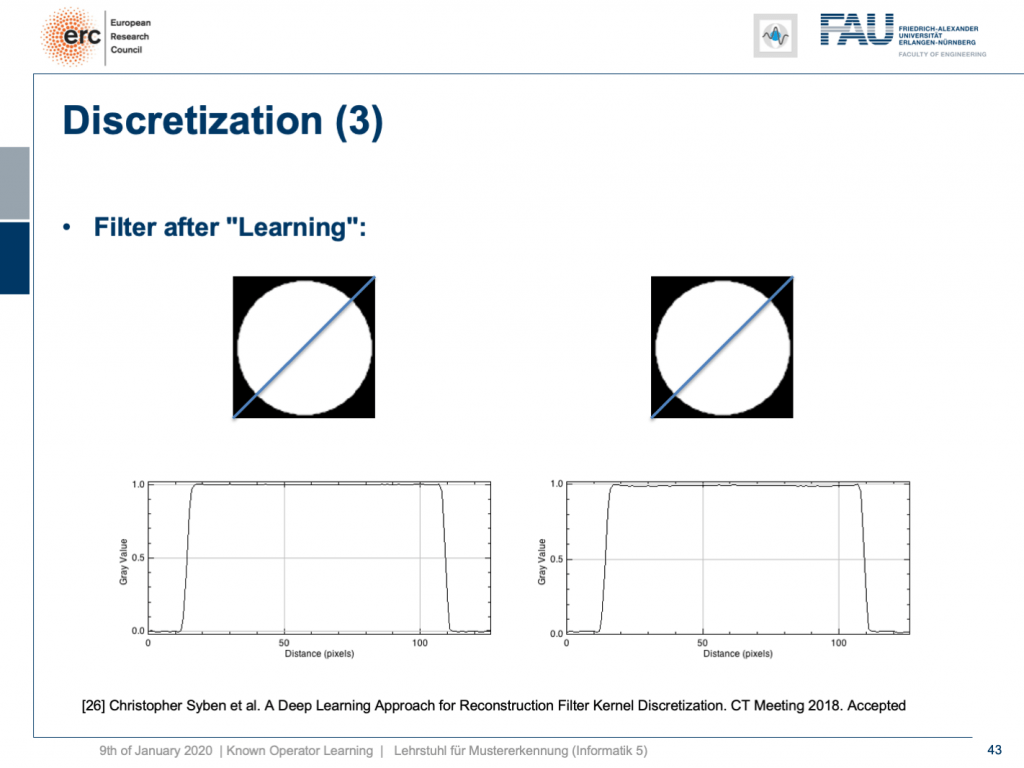
What happens if you do and then? Well, naturally, after learning the artifact is gone. So, you toilet remove this artifact. Well, this is kinda an theoretical example. We also have some more.
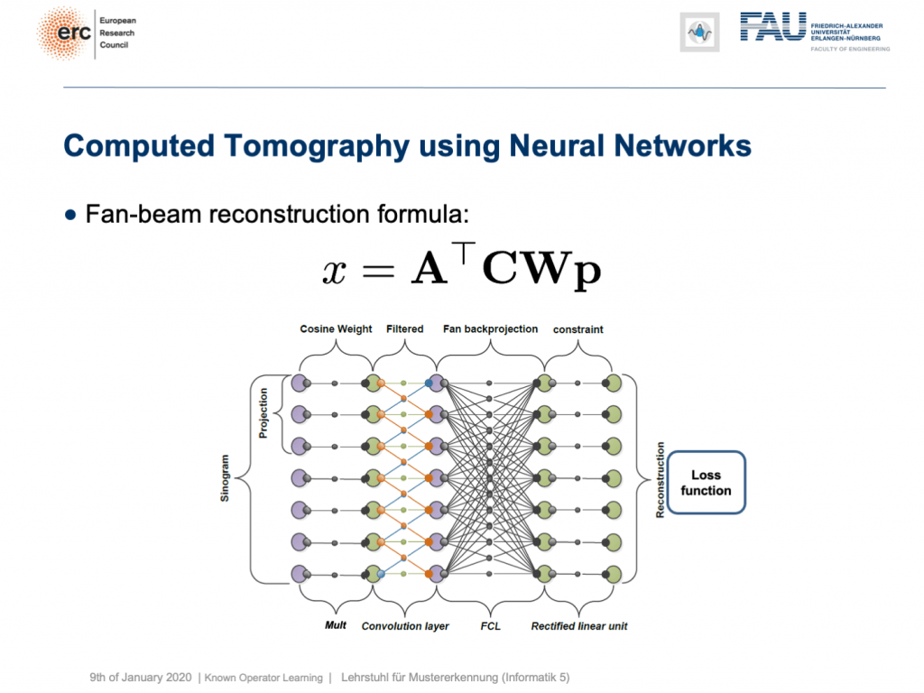
You arse see that you can approximate also fan-beam reconstruction with replaceable matrix kinds of equations. We experience now an additive ground substance W. So, W is a point-wise weight that is multiplied to to each one pixel in the input image. C is now directly our convolutional matrix. So, we rear describe a fan-beam reconstruction formula simply with this equation and of course, we can produce a resulting network impossible of this.
Straight off let's view what happens if we come back to this limited lean on tomography job. So, if you have a complete read, it looks like this. Net ball's go to a scan that has only 180 degrees of rotation. Here, the borderline gear up for the skim would be in reality 200 degrees. Sol, we are lacking 20 degrees of rotation. Non as strong as the limited angle problem that I showed in the intro of notable operator learning, but soundless significant artifact emerges here. Now, let's take as pre-grooming our traditional filtered back-projection algorithmic rule and adjust the weights and the whirl. If you do so, you get this reconstruction. And so, you can see that the image superior is dramatically improved. Much of the artifact is done for. There are still or s artifacts on the right-hand side, but image quality is dramatically healthier. Now, you could argue "Well, you are again exploitation a black box!".
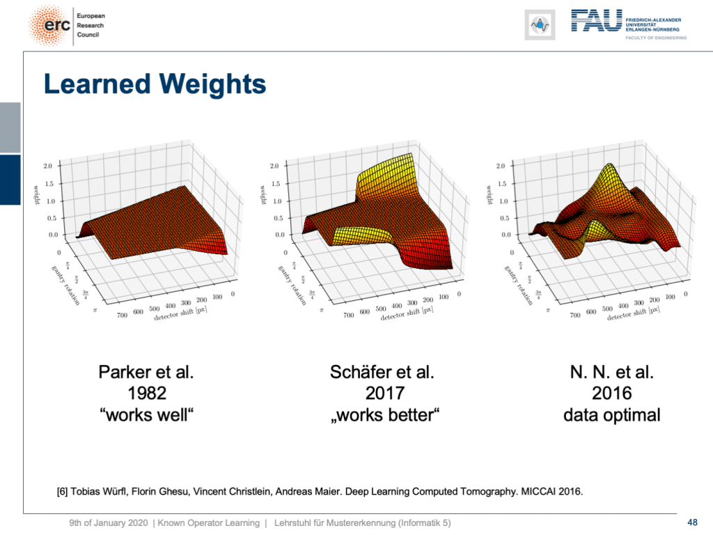
but that's non actually harmonious because our weights can be mapped hindmost into the original interpretation. We still bear a filtered back-projection algorithmic rule. This substance we can record out the housebroken weights from our network and compare them to the submit-of-the-art. If you bet here, we initialized with the so-known as Parker weights which are the solution to a short scan. The idea Hera is that opposing rays are assigned a weight such that the rays that measure exactly the same line integrals essentially sum adequate one. This is shown on the left-hand side. On the straight-hand side, you find the solution that our somatic cell meshing found in 2022. So this is the data-optimum solution. You see it did significant changes to our Parker weights. Now, in 2022 Schäfer et al. published a heuristic rule how to fix these limited angle artifacts. They suggested ramping sprouted the weight of rays that eat the area where we are absent observations. They simply increase the weight in order to fix the deterministic mass loss. What they found looks best, simply is a heuristic. We can see that our neural meshwork found a very similar solution and we can demonstrate that this is data-optimal. Soh, you can see a distinct difference on the rattling unexpended and the very light right. If you look here and if you look present, you tin can see that in these weights, this goes the whole way up here and here. This is in reality the end of the detector. So, here and here is the bounds of the detector, likewise Hera and here. This means we didn't have whatever variety in these areas here and these areas here. The reason for that is we never had an objective in the grooming information that would fulfil the entire detector. Thu, we can also not backpropagate gradients here. This is why we essentially have the original low-level formatting still at these positions. That's pretty cool. That's in truth interpreting networks. That's very understanding what's happening in the training process, right-hand?
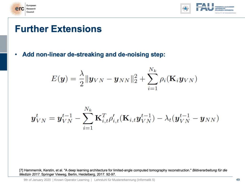
Sol, can we do more? Yes, there are even other things like so-called variational networks. This is work by Kobler, Pock, and Hammernik and they basically showed that any sort of energy minimization backside be mapped into a kind-hearted of unrolled, feed-forward problem. Thus, essentially an energy minimization lav be solved by slope lineage. So, you fundamentally cease ascending with an optimisation problem that you seek to minimize. If you want to do that efficiently, you could essentially formulate this as a recurrent neural net. How did we get by with recurrent neural networks? Well, we unroll them. So any kind of energy minimization can be mapped into a feed-impertinent neural mesh, if you fix the number of iterations. This way, you behind then take an energy minimization like this iterative reconstruction formula here or iterative denoising formula here and figure its gradient. If you do so, you will essentially end up with the previous image configuration minus the negative gradient direction. You do that and repeat this step by ill-trea.
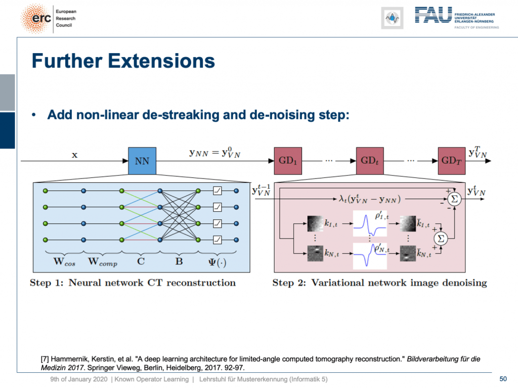
Hither, we have a special solution because we combine IT with our somatic cell network reconstructive memory. We just want to learn an image sweetening gradation after. So what we do is we take our neural network reconstruction so bait up connected the previous layers. In that respect are T streaking or denoising steps that are trainable. They use compressible sensing theory. So, if you want to check into more details here, I recommend taking one of our image Reconstruction Period classes. If you flavor into them you can see that there is this mind of compressing the image in a distributed domain. Hither, we show that we can actually learn the transform that expresses the image table of contents in a sparse arena pregnant that we can also get this bran-new sparsifying transform and interpret information technology in a traditional signalise processing sensation.
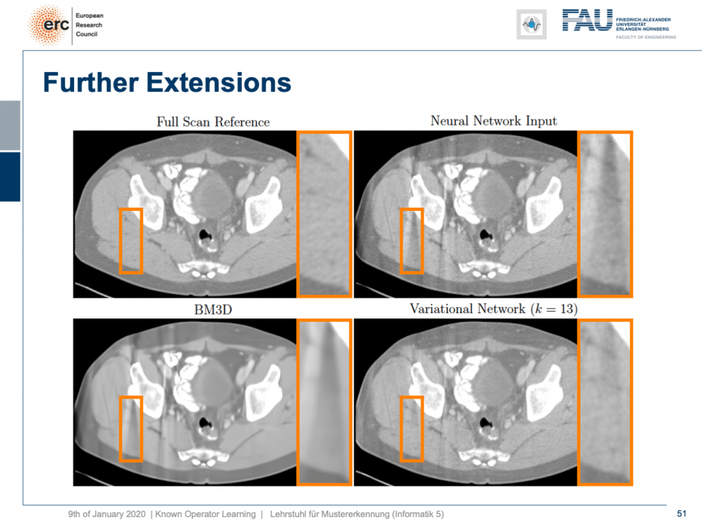
Army of the Righteou's appear at some results. Here, you can visualise that if we take the full scan reference, we get really an artefact-freeborn pictur. Our neural net output with this reconstruction network that I showed earlier kinda is improved, simply it placid has these streak artifacts that you see happening the overstep right. Along the bottom left, you see the output of a denoising algorithmic program that is 3-D. So, this does denoising, but it still has problems with streaks. You can picture that in our variational Meshwork connected the bottom right, the streaks are rather a bit suppressed. Soh, we really learn a transubstantiate founded on the ideas of compressed sensing in order to remove those streaks. A very prissy system network that mathematically on the button models a compressed sensing reconstruction approach shot. So that's exciting!
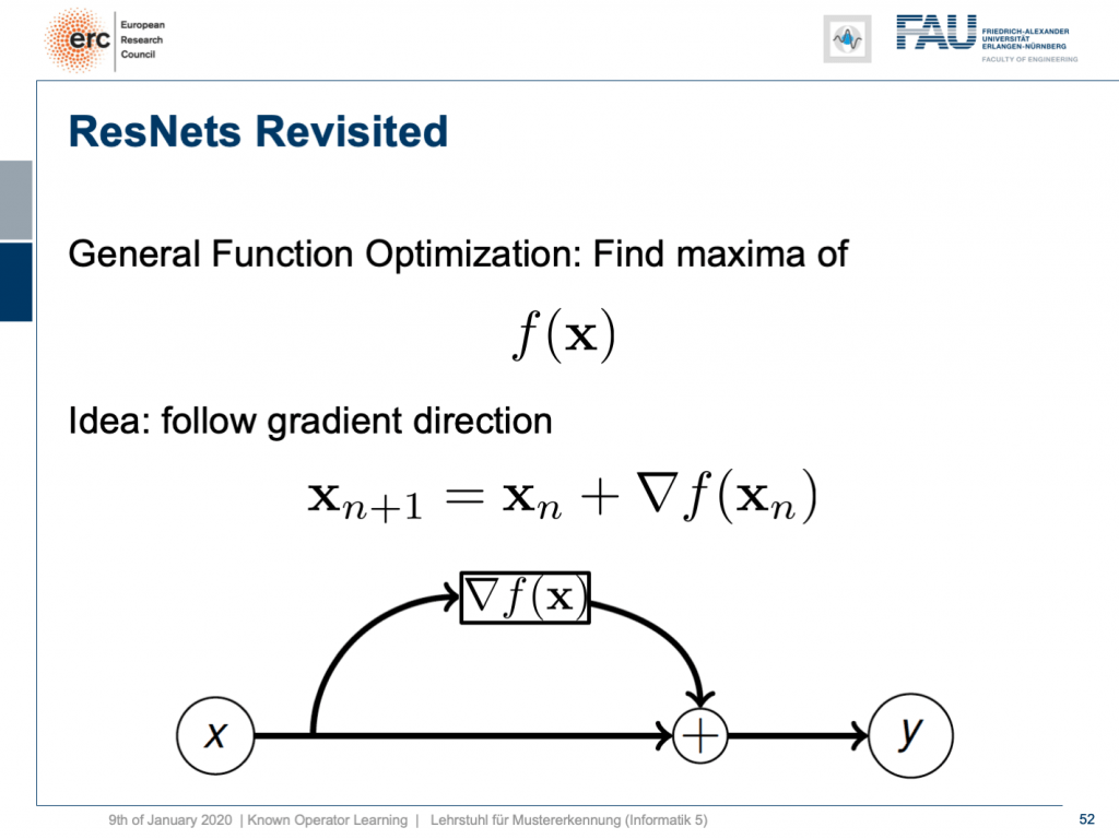
Past the way, if you think of this muscularity minimization idea, then you as wel find the following rendering: The vigour minimization and this unrolling always lead to a ResNet because you take the late form minus the minus gradient direction meaning that it's the old layers output plus the new layer's configuration. So, this essentially means that ResNets can also be expressed in that kind of way. They always are the result of any kind of energy minimization problem. It could also live a maximization. Anyhow, we don't even stimulate to know whether it's a maximation surgery minimisation, but generally, if you have a function optimisation, then you can always find the solution to this optimization process through a ResNet. Soh, you could argue that ResNets are likewise proper to find the optimisation strategy for a completely unknown erroneous belief purpose.
Interesting, isn't information technology? Well, there are a twain of more things that I want to order you about these ideas of noted operator eruditeness. Besides, we wish to assure more applications where we throne apply this and maybe also both ideas on how the field of deep learning and machine learning will evolve over the incoming couple of months and years. So, give thanks you very much for listening and see you in the next and final video. Au revoir!
If you likeable this post, you can find more essays here, more educational material on Machine Learning here, or have a look at our Deep LearningLecture. I would likewise appreciate a follow on YouTube, Twitter, Facebook, or LinkedIn in case you want to be informed active more essays, videos, and research in the future. This article is released under the Creative Commons 4.0 Attribution License and stern live reprinted and modified if referenced. If you are interested in generating transcripts from picture lectures try AutoBlog.
Thanks
Many thanks to Weilin Fu, Florin Ghesu, Yixing Huang Christopher Syben, Marc Aubreville, and Tobias Würfl for their support in creating these slides.
References
[1] Guilder Ghesu et al. Robust Multi-Plate Anatomical Landmark Detection in Incomplete 3D-CT Data. Medical Image Computer science and Reckoner-Assisted Intervention MICCAI 2022 (MICCAI), Quebec, Canada, pp. 194–202, 2022 — MICCAI Young Research worker Grant
[2] Florin Ghesu et Camellia State. Multi-Scale Deep Reinforcement Learning for Period 3D-Landmark Detection in CT Scans. IEEE Transactions on Pattern Psychoanalysis and Machine Intelligence activity. ePub ahead of print. 2022
[3] Bastian Bier et al. X-ray-transmute Invariant Anatomical Landmark Detection for Pelvic Injury Surgery. MICCAI 2022 — MICCAI Teenaged Researcher Honour
[4] Yixing Huang et Camellia State. Some Investigations connected Robustness of Intense Learnedness in Limited Angle Tomography. MICCAI 2022.
[5] Andreas Maier et atomic number 13. Precision Learning: Towards wont of known operators in neural networks. ICPR 2022.
[6] Tobias Würfl, Florin Ghesu, Vincent Christlein, Andreas Maier. Deep Learning Computed Tomography. MICCAI 2022.
[7] Hammernik, Kerstin, et Alabama. "A deep encyclopaedism architecture for limited-angle computed tomography reconstruction." Bildverarbeitung für give out Medizin 2022. Springer Vieweg, Irving Berlin, Heidelberg, 2022. 92–97.
[8] Aubreville, Marc, et al. "Inscrutable Denoising for Deaf-aid Applications." 2022 16th International Shop on Natural philosophy Bespeak Sweetening (IWAENC). IEEE, 2022.
[9] Christopher Syben, Bernhard Stimpel, Jonathan Lommen, Tobias Würfl, Arnd Dörfler, Andreas Maier. Deriving Neural Network Architectures victimization Precision Scholarship: Latitude-to-fan beam Conversion. GCPR 2022. https://arxiv.org/abs/1807.03057
[10] Fu, Weilin, et alii. "Frangi-net." Bildverarbeitung für become flat Medizin 2022. Springer Vieweg, German capital, Heidelberg, 2022. 341–346.
[11] Fu, Weilin, Lennart Husvogt, and Stefan Ploner James G. Maier. "Lesson Learnt: Modularization of Artful Networks Allow Cross-Modality Reuse." arXiv preprint arXiv:1911.02080 (2019).
A Convolutional Framework for Forward and Back Projection in Fan Beam Geometry
Source: https://towardsdatascience.com/known-operator-learning-part-3-984f136e88a6

